What’s nice about the filters in Google Sheets is that you can create Filter Views and reuse them. Then anytime you want to make that certain data jump out at you, just select the Filter View. Here, we’ll show you how to use Filter Views in Google Sheets to help you work with your spreadsheets easier.
Create a Filter
You can create a temporary filter for your data in Google Sheets. Then, if you find yourself using that same filter, again and again, save it as a Filter View.
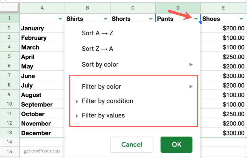
Select Filter Options
As mentioned in Step 3 above, you can filter your data by three variables: color, condition, or value. You can also use the Search box for very specific data. Here’s how each option works. Color: If you apply a fill color to a cell or font color to text, you can filter by color. This option does apply to colors used for conditional formatting in Google Sheets, but not to alternating colors in your sheets.
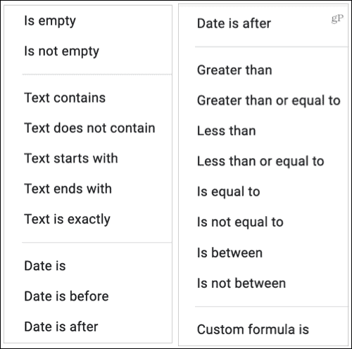
Condition: Choose a condition to apply to your data to filter by. You can use conditions for text (contains, does not contain), dates (is before, is after), numbers (equals, is less than), empty cells, or custom formulas.
Value: Select from values that appear in that column. Check or uncheck, or use the Select All or Clear options.
Search: Use the Search box to find a specific piece of data in the column to filter by.
As a reminder that your data has a filter, you’ll see the icon in the column header turn to a solid (filled in) filter icon.
Turn Off a Filter
To remove a temporary filter, click Data > Turn Off Filter from the menu use the Filter button in the toolbar.
Save the Filter as a View
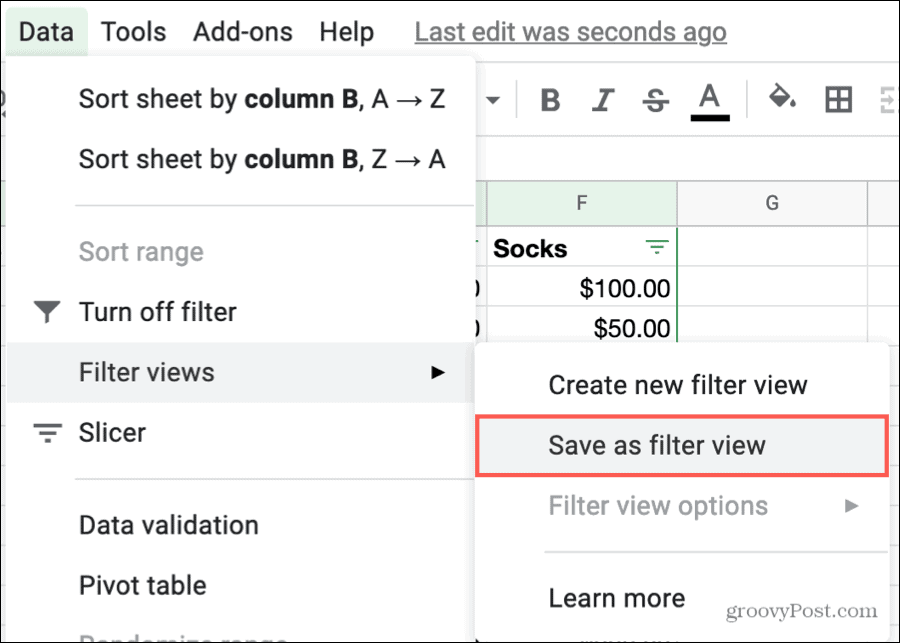
To save a temporary filter as a Filter View that you can use again, click Data > Filter views > Save as filter view.
You’ll then see the sheet transform to include a black bar across the top of it to denote the Filter View. In that bar, you can change the filter name or cell range, duplicate, or delete the Filter View. Name: Click the box next to Name or the Options button (gear icon) and pick Rename. Range: Click the box next to Range or the Options button and pick Update Range. Duplicate or Delete: Click the Options button and pick either Duplicate or Delete.
You can also click Data > Filter views > Filter view options in the menu to change any of the above.
Tips for Creating Filter Views
Filter Names: Since you can create more than one Filter View for your sheet, giving them meaningful names is helpful for selecting the one you need.Saving Views: When you make changes to a Filter View, your changes are saved automatically. So, if you want to start with an existing Filter View that you simply update, use the Duplicate action for a quick start.New Filter Views: You may know before you apply a temporary filter that you want to save it as a Filter View. If so, you can select Data > Filter views or click the Filter button in the toolbar and pick Create new filter view.Sharing Your Sheet: If you’re sharing a spreadsheet in Google Sheets, anyone with access can see and use your Filter Views. Only those with permission to edit the sheet can change those Views.Viewing a Shared Sheet: If you have permission to view (not edit) another person’s sheet, you can only create temporary filters. You cannot save Filter Views.
Use Your Filter Views
Anytime you want to apply a Filter View you have saved, click Data > Filter views or use the Filter button in the toolbar and select its name.
When you finish viewing your data with a filter, click the X on the top right of the Filter View to close it. Your sheet will return to normal, displaying all your data without any filters applied.
See the Data You Need With Filter Views in Google Sheets
By using filters, you can see only the data you need when you’re using your sheet. And with Filter Views that you can reuse, you save time because you don’t have to keep setting up and applying temporary filters. For more help analyzing your data, check out how to get quick column statistics in Google Sheets. Comment Name * Email *
Δ Save my name and email and send me emails as new comments are made to this post.
![]()


![]()


