This is because an IF statement lets you check multiple conditions, and then use a different calculation based on that check. In this article, you’ll learn the basic structure of an IF statement and several examples that’ll show you how to use them effectively.
How to Use the IF Statement
An IF statement is made up of three different parts.
A logical expression using one of several comparison operatorsThe result to return if the comparison is trueThe results to return if the comparison is false
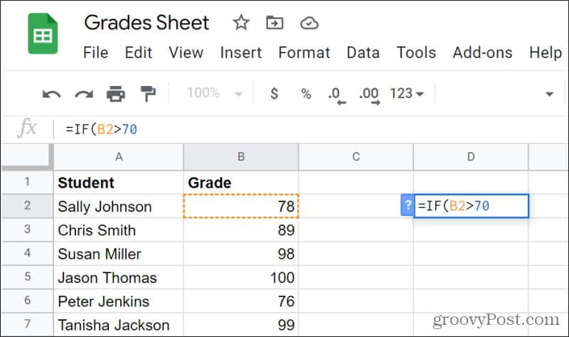
The results in the cell are determined based on the comparison. If you fill the row underneath the IF statement, the cell references update and perform the same comparison and provide results for all of the data in the referenced cells. As a simple example, consider a spreadsheet of student names and grades. You can use an IF statement to display a “C” letter grade if the numerical grade is over 70. The first part of the IF statement is the logical expression.
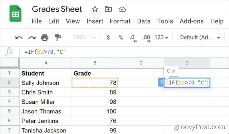
In this example, the expression checks to see if cell B2 is greater than 70. To add the next part of the statement, type a comma (,). Then provide what should be returned if the comparison is true (B2 is greater than 70). In this case, that’ll be the string “C”.
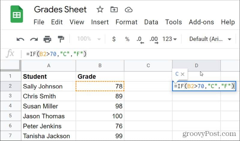
Next, type a comma and provide the last parameter for the IF statement. This will be the result if the expression is false (B2 is less than 70).
This last parameter will return an “F” string if the number is less than 70. This isn’t really a practical example because it’ll only check for C or F grades and no other, but it’s a basic example of how the IF function works.
IF Statement Considerations
IF statements work for different data types, both the comparison and the results.
You can compare string values. For example: “IF(A2=”ON”,”True”,”False”)” returns a “True” string if the cell A2 contains the string “ON”, and “False” otherwise.You can compare numeric values. For example: “IF(A2>=0,”Positive”,”Negative”)” returns a “Positive” string if A2 is greater than zero, and “Negative” otherwise.Return string or numeric values as outputs. To do this: “IF(A2>=0,1,2) will return a 1 if A2 is greater than zero, and 2 otherwise.
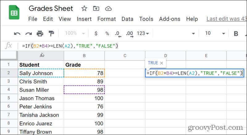
You can also do more complex statements with calculations on either side of the operator. These can include mathematical calculations, or additional Google Sheets functions that return values or strings.
Just make sure that the returned values on each side of the comparison operator are the same. Otherwise, you could end up trying to compare a string result to a numeric result, and you’ll see an error instead of a result.
Nesting IF Statements
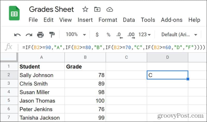
Another useful way to use IF statements is by nesting them together to do more complex comparisons across even more cells. Here’s how this works: IF(first_comparison, true_result, IF(second_comparison, true_result, false_result)) The logic of these IF statements work in steps. The first comparison happens, and if it’s true the true result gets displayed and the statement logic is finished. If the first comparison is false, the second comparison takes place, and so on. Going back to the grade spreadsheet example, you could write a full nested IF statement for all grades from A through F. This is what that IF statement would like for this sample spreadsheet: =IF(B2>=90, “A”, IF(B2>=80, “B”, IF(B2>=70, “C”, IF(B2>=60, “D”, “F”)))) When you press Enter, you should see the correct letter result in the cell where you typed the formula.
When you use this kind of logic, it’s important to choose your first comparison at the very top of the range if you’re using a > operator, or the bottom of the range if you’re using a < operator. This way the false comparison will only be used for the next item in the range in the correct order.
Using AND or OR
One other approach that can be useful is setting strict bounds on your comparisons using AND or OR operators. In the grades example, you can ensure an “A” is only applied for any numerical grade between 100 and 90 by using an AND statement. Keep in mind that the AND statement in Google Sheets starts with the word “AND” and then the two conditions inside the parenthesis. For example, for an A grade, the comparison would be: =IF(AND(B2>=90,B2<100),“A”,”Not A”) Obviously, you wouldn’t want to display “Not A” if the grade is less than 90, so you’d need to insert another IF statement in that position as described in the previous section. The full nested IF statement for all grades from A through F would look like this: =IF(AND(B2>=90,B2<100),“A”,IF(AND(B2>=80,B2<90),“B”,IF(AND(B2>=70,B2<80),“C”,IF(AND(B2>=60,B2<70),“D”,“F”)))) This formula can look intimidating when you type it into Google Sheets, but it works!
Why would you use this approach rather than just an upper-end comparison (such as “>=90” for A, “>=80” for B, and so on)? Using AND and OR is best reserved for cases where you need to make sure the result you want to display falls within an absolute range with two limits. It isn’t always necessary to get the right results, but in some cases, if you don’t include these operators, the results could be unpredictable.
The Value of IF Statements in Google Sheets
Most other functions in Google Sheets provide a single result for a single function. The IF statement lets you add some intelligence and decision-making to your functions. And by adding additional functions like AND or OR into the mix, your IF statement functions can be as complex and useful as you like. For very complicated nested IF statements, it’s useful to write out all parts of the function in an app like Notepad so that you can organize each piece. This also ensures that you use the right number of closing parenthesis at the end of your statement, and avoid getting any errors in your results. Comment Name * Email *
Δ Save my name and email and send me emails as new comments are made to this post.
![]()

